Dremel is a scalable, interactive ad-hoc query system for analysis of read-only nested data.
Data Model
The data model is based on strongly-typed nested records. The abstract syntax is given by:
τ = dom | <A1 : τ[*|?],…,An : τ[*|?]>
where τ is an atomic type or a record type. Atomic types in dom comprise integers, floating-point numbers, string, etc. Records consist of one or multiple fields. Field i in a record has a name Ai and an optional multiplicity label. Repeated field (*) may occur multiple times in a record. Optional field (?) may be missing from the record. Otherwise, a field is required, must appear exactly once.
Nested Columnar Storage
In this section, we address the following challenges: lossless representation of record structure in a columnar format, fast encoding and efficient record assembly.
Repitition and Definition Levels
Values alone do not convey the structure of record. Given two values of a repeated field, we do not know at what ‘level’ the value repeated. Likewise, given a missing optional field, we don’t know which enclosing records were defined explicitly. We therefore introduce the concepts of repetition level and definition level.
Repetition Levels
Taking following schema tree and sample records as examples:
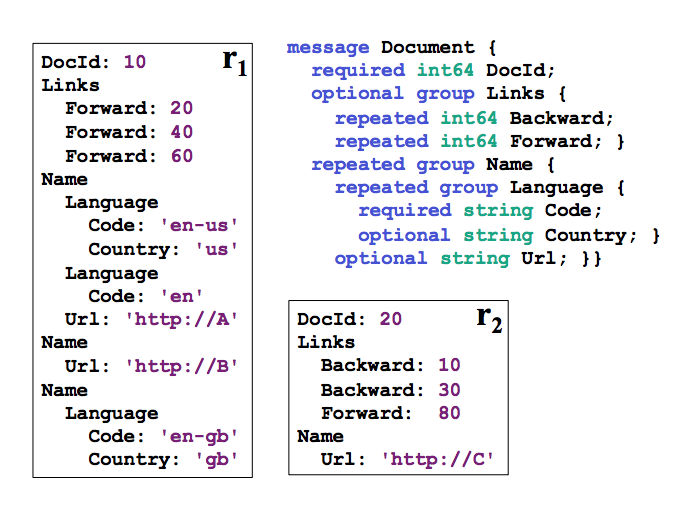
Considering field Code. It occurs three times in r1. To diambiguate these occurences, we attach a repetition level to each value. It tells us at what repeated field in the field’s path the value has repeated. A more straightforward explanation would be the LCA of current and previous occurence in the data tree. The field path Name.Language.Code contains two repeated fields, Name and Language. Hence, the repetition level of Code ranges between 0 and 2; level 0 denotes the start of a new record. The repetition levels of Code values in r1 are 0 (New record),2 (Language),1 (Name).
Notice that the second Name in r1 doesn’t contain any Code values. To determine that ‘en-gb’ occurs in the third Name instead of the second, we add a NULL value between ‘en’ and ‘en-gb’ in the columnar table (see figure below). Code is a required field, in Language, so the fact that it is missing implies that Language is not defined. In general, determining the level up to which nested records exist require extra information.
Definiiton Levels
Each value of a field with path p, esp. every NULL, has a definition level specifying how many fields in p that could be undefined (because they are optional or repeated) are actually present in the record. To illustrate, observe that r1 has no Backward links. However, field Links is defined (at level 1). To preserve this information, we add a NULL with definiiton level 1 to the Links.Backward column. Similarly, the missing occurence of Name.Language.Country in r2 carries a definition level 1, while its missing occurences in r1 have definition levels 2 (inside Name.Language) and 1 (insideName`), respectively.
We use integer definition levels as opposed to is-null bits so that the data for a leaf field contains the information about the occurences of its parent fields.
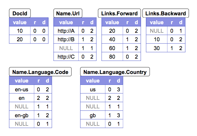
The repitition and definition levels of sample records are listed below:
Encoding
Each column is stored as a set of blocks. Each blocks contains the repetition and definitionlevels (henceforth, simply called levels) and compressed field values. NULLs are not stored explicitly as they are determined by the definition levels: any definition level smaller than the number of repeated and optional fields in a field’s path denotes a NULL. Definition levels are not stored for values that are always defined (all required along field’s path). Similarly, repetition levels are stored only if required; for example, definition level 0 implies repetition level 0 (all required fields in path). Levels are packed as bit sequence. We only use as many bits as necessary; for example, if max definition level is 3, we use 2 bits per definiiton level.
Splitting Records into Columns
The next challenge we address is how to produce column stripes with repetition and definition levels efficiently.
The actual algorithm is straightforward, both levels can be calculated when traversing the data tree. Assuming we are scanning records in the data tree, if a field is repeated, then each instance will also be scanned also:
- Definition level will just be calculating how many optional / repeated in the field’s path.
- For repitition level, we will need to keep track of fields we have seen on that recursion level. If a field is visited, then its repetition level will be equal to its parent (not seen yet) or number of repeated fields (seen) on its path.
Many datasets used at Google are sparse. Hence we try to process missing fields as cheaply as possible. To produce column stripes, we create a tree of field writers, whose structure matches the field hierarchy in the schema. The basic idea is to update field writers only when they have their own data, and not try to propagate parent state down the tree unless absolutely necessary. To do that, child writers inherit the levels from their parents. A child writer synchronizes to its parent’s level whenever a new value is added. Child writer level could get out of sync when encoutering NULL value.
Record Assembly
Given a subset of fields, our goal is to reconstruct the original records as if they contained just the selected fields, with all other fields striped away. That is one of the major advantage of columnar storage becuase we don’t need to scan the whole row. The key idea is this: we create a finite state machine (FSM) that reads the field values and levels for each field, and appends the values sequentially to the output records. State transitions are labeled with repitition levels. Once a reader fetches a value, we look at the next repetiiton level to decide what next reader to use. The FSM is traversed from the start to end state once for each record.
The FSM essentially represent which column to read based on the next repitition level of current field. To describe the algorithm, we introduce the concept of barrier level, which is the repitition level of the LCA of current field and next field in the sequence of proto. Because the most crucial step is to determine whether to move to the next field or a previous field. For a given field, the repetition level of next instance can range from [0, maxLevel]:
- If the next repetition level of current column is between [0, barrierLevel], go the the next field in schema tree.
- If the next repetition level of current column is between [barrierLevel + 1, maxLevel], for each parent field in field path whose repetition level is larger than the barrier level, set transition (field, backLevel) -> parent leftmost leaf field.
Barrier level is important here, because any repetiition level larger than it indicate the current column / field is still repeating under this LCA, which means we shouldn’t go to the next column / field in the schema tree. Instead, it should go back to the parent with the same repetition level as the next instance in the columnar storage, and start constructing that parent field again with leftmost leaf node.
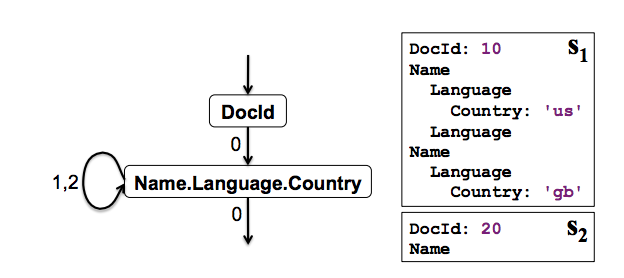
The FSM of Document proto is as below:

Taking Name.Language.Country as an example, its repetiition level can range between [0, 2], and the barrier is Name.Url, the LCA is Name which indicates the barrier level is 1. So if the next repetition level of Name.Language.Country is 2, it means it still repeats under Name.Language so it should go back to the leftmost leaf under Name.Language, which is Name.Language.Code. Otherwise, it indicates it repeats under Name or a new record, so we can go to Name.Url.
If only a subset of fields need to be retrieved, we construct a simpler FSM that is cheaper to execute. The image below depicts an FSM for reading the fields DocId and Name.Language.Country.
Query Language
Dremel’s query language is based on SQL and is designed to be efficietly implementable on columnar nested storage. Each SQL statement (and algebraic operators it translates to) takes as input one or multiple nested tables and their schemas and produces a nested table and its output schema.

To explain what the query does, consider the selction operation (the WHERE clause). The selection operator prunes away the branches of the tree that do not satisfy the specified conditions. Thus, only those nested records are retained where Name.Url is defined and start with http. Next, consider projection. Each scalar experssion in the SELECT clause emits a value at the same level of nesting as the most-repeated input field used in that expression. The COUNT expression illustrate within-record aggregation. The aggregation is done WITHIN each Name subrecord, and emits the number of occurences of Name.Language.Code for each Name as a non-negative 64-bit integer (uint64).
Query Execution
We discuss the core ideas in the context of a read-only system, for simplicity. Many Dremel queries are one-pass aggregations; therefore, we focus on explaining those.
Tree Architecture
Dremel uses a multi-level serving tree to execute queries (see image below). A root server receives incoming queries, reads metadata from the tables, and routes the queries to the next level in the serving tree. The leaf servers communicate with the storage layer or access the data on local disk. Consider a simple aggregation query below:
1 | SELECT A, COUNT(B) FROM T GROUP BY A |
When the root server receives the above query, it determins all tablets, i.e., horizontal partitions of the table, that comprise T and rewrites as the query of union of results of all sub queries.
Each serving level performs a similar rewriting. Ultimately, the queries reach the leaves, which scan the tablets in T in parallel. On the way up, intermediate servers perform a parallel aggregation of partial results.
Query Dispatcher
Dremel is a multi-user system, i.e., usually several queries are executed simultaneously. A query dispatcher schedules queries based on their priorities and balances the load. Its other important role is to provide fault tolerance when one server becomes much slower than others or a tablet replica becomes unreachable.
The amount of data procesed in each query is often larger than the number of processing units available for execution, which we call slots. A slot corresponds to an execution thread on a leaf server. During execution, the query dispatcher computes a histogram of tablet processing times. If a tablet takes a disproportionately long time to process, it rechedules it on another server. Some tablets may need to be redispatched multiple times.
Each server has an internal execution tree, as depicted on the right-hand side of the image above. The internal tree corresponds to a physical query execution plan, including evaluaiton of scalar expressions. An execution plan for project-select-aggregate queries consists of a set of iterators that scan input columns in lockstep and emit results of aggregates and scalar functions annotated with the correct repetition and definition levels, bypassing record assembly entirely during query execution.