Paper Reading: Dremel 2

In previous article, we have introduced the columnar storage of Dremel. In this paper summary, we will focus on running query on tree structure records in Dremel.

Data

The data types are defined recursively as:

1. A tuple type is a list of attribute names and a (previously defined) type for each attribute.
2. The type of an attribute is either a basic type or a tuple type. Further, attributes within a tuple type can be either required, optional, repeated, or required and repeated.
3. A relation type is a repeated tuple type. We shall refer to the type of tuples (unrepeated) as the schema of the relation.

Representing Schemas

We use the conventional notation for types. For example, int and string will denote the basic types integer and strings. A tuple type T with attributes A₁,…, A_n whose types are T₁,…, T_n, respectively will be denoted:

T = {A₁ : T₁,…, A_n : T_n}

The repeated type T will be denoted T^*, the optional type T will be denoted T?; we also use T⁺ to denote “one or more occurrences.”

We shall use trees to represent schemas. The following rules define how a tree is constructed from a data type:

1. A node that represents a tuple type has children for each attribute of that tuple type, in order from the left.
2. The children are labeled by their corresponding attribute names.
3. In addition, each attribution has a repetition constraint. A repeated attribute is labeled with a *; an optional attribute is labeled with a ?, an attribute that is required and repeated is labeled by a +.
4. The root itself is labeled by the name of the type. Typically, the root type is starred, since it is the type of a relation and the relation consists of zero or more tuples of the root type.
5. Leaf nodes are of basic type.

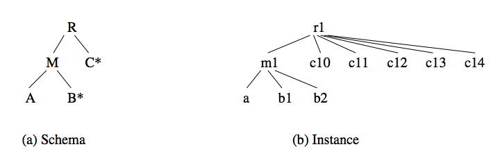
For example, the schema tree above for a hypothetical data type represents advertisers at a search engine.

Instances of a Schema

An instance of a data type or schema consists of replacement of each subtype by an appropriate number of instances of that subtype. More formally:

1. An instance of a basic type is any single value of the appropriate type.
2. An instance of a tuple type is a node whose children are each instances of one of the types of one of its attribute.

The image below suggests a possible instance of the relation that is described by the schema tree above.

Dummy Occurrences

For several reasons, including the way we flatten instances (see section below), we shall maintain a fiction about attributes that are repeated or optional. We imagine that there is one dummy occurence of this attribute, all of whose descendant leaves have the value NULL. Since this instance may have descendant interior nodes representing repeated or optional groups, those descendants are consequently treated as if they had only the dummy instance.

We do not show this dummy instance in the tree diagrams, although as we shall see, there are reasons why it is useful to imagine it is there, and able to appear when needed. For instance, when we discuss querying, we shall see that sometimes all the occurences of some repeated attribute are deleted. We do no want anything else in the tree to disappear, so we replace the deleted occurences by the dummy occurrence. This viewpoint is consistent with the treatment of tree-structure instances as an outerjoin of conventional relations.

Querying Tree-Structured Data

A more recent approach to query languages attempts to be more SQL-like, and to think of the instances of a tree data type as if they were tuples of a relation.

Flattening

Flattening has always been regarded as a fundamental algebraic operation on nested relations. Informally, we flatten an instance of a tree data type by selecting one from each repeated group of values in all possible ways. This selection is made independently at all levels.

Since filtering (selection) queries can delete all occurrences of repeated or optional attribute, we are going to want to make explicit the effect of the dummy occurrences discussed above. Thus, we define the “full flattening” (or just “flattening” when there is no ambiguity) of a tree instance to include all the tuples that result when we include all dummy instances in the flattening. To save space, we can remove those rows that are subsumed by another tuple of the flattened table. A roa r1 is subsumed by row r2 agrees with r1 wherever r1 is not NULL. We call this relation the reduced flattening of the tree.

More formally, if I is an instance of some schema, we define the (ordinary) relation flatten(I) recursively as follows:

1. If I is a single element of basic type, then flatten(I) is the tuple with a single component; that component is the value of I.
2. If I is an instance of some tuple type with attributes A₁,…, A_n: Divide the children of the root of I into n groups, such that the first group is all the nodes that are occurrences of A₁, the second group is all the occurrences of A₂, and so on. For the ith group, construct a relation R_i that has attributes for all leaves of the schema tree rooted at A_i, as follows:
   a. Recursively apply the flatten operation to the instance represented by each node in the group for A_i. However, if A_i is repeated or optional, include the dummy instance in this set of instances.
   b. Take the union of the relation produced for each instance. The union is the relation R_i.
3. Finally, to get the relation flatten(I), take the Cartesian product R₁ x … x R_n.

Let us see how to flatten the instance in data tree above.

The image above we present the flattening of the part of the instance with root at a1. The relation for ca1 is the cartesian product of the relation for i1, the relation for bu1, the union of the relations for s1 and s2 and, the union of the relations for cl1, cl2, and cl3. The result appears in row1 through 25. Similarly, for ca2, the result appears in rows 26 through 30.

Finally, to construct the relation for a1, we take the product of the relations n1 and e1. The result looks similar to the image above but there are two new attributes (Name and Email) at the left.

Filter Queries

A filter is a conjunction of comparisons AθB where A is an attribute, B is an attribute or a constant and θ can be any comparison for which given two values the outcome is “true” or “false.”

Querying Flattened Data

Flattening the tuples and apply the query to the ordinary relation that results. There are two problems with this idea:

1. Flattening can expand greatly the amount of space needed to hold a tuple.
2. When you flatten a tree and then apply some filter to the resulting relation, it is common for there to be no way to prune the original tree to yield a tree that would have produced the result of the filtering the flattened relation.

It is the purpose of this paper to resolve these two problems by:

1. Investigating when the result of filtering a flattened relation is what we get by pruning the tree then flattening.
2. Giving an algorithm to perform the filtering on the tree itself, whenever it is possible to do so.

To see the problem concretely, consider the schema in figure below and an instance of that schema. The values of B and C are integers, but we give each occurrence of a B-value or C-value a name, such as b₁, to make clear which attribute, B or C, each integer comes from. Suppose we apply to the instance of figure the query:

SELECT B, C FROM A WHERE B < C

This example can be used to explain why we need a flattened relation where NULL’s appear. We apply this query to the flattened version, which is shown in image below. Note that relation (a) is a reduced flattened version, since we have not shown the tuple where one or both of B and C are NULL. However, in this case, the result would not change if we consider the full flattening. We shall see in section below where it becomes essential to use the full flattening.

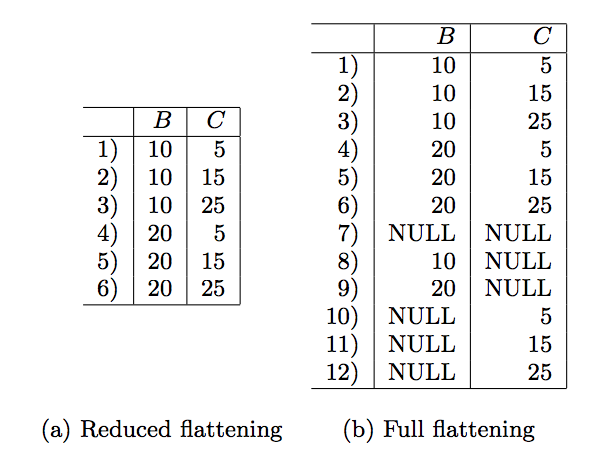
Notice that the second, third and sixth tuples satisfy the filter. Thus, the result of this query is shown below. However, this relation is not the flattening of any tuple with the schema. To see why, notice that such a tree-structured tuple would have B-values 10 and 20 and also have C-values 15 and 25.But the flattening of the tree would also yield the tuple (20, 15). We conclude that this SQL query cannot be executed on tree-structured tuple; it can only be executed on the flattened version of the tree, and the result has a schema differernt from the schema of the input tuples.

Handling NULL’s in Query Execution

Now, using the same schema and instance, suppose we have the query:

SELECT * FROM A
WHERE B = 10 AND C = 35;

According to the tree-pruning algorithm, the data leaves that do not satisfy the filter will be deleted. Thus the output data tree has only one leaf for attribute B (10) and not leaves for attribute C. The flattening, thus, contains only the row (10 NULL).

But if we aply the query to the reduced relation (a) above, we get no tuples. Possibly, we could resolve the problem by starting with the full flattening (b), because that table has the necessary NULL’s. But according to the SQL standard, the truth value of C = 35 is UNKNOWN when C is NULL, which is not true enough.

The resolution to this dilemma, we believe, is to deviate from the SQL standard by allowing UNKNOWN to be “suffcient true” to allow a row to reach the result of the query. If we do so, then rows 7 and 8 of full flattening (b) pass the filter. However, when we reduce the relation, row 7 is subsumed by row 8, so we get only the latter row as the answer.

The Dominance Relation

Now, we are going to show how to distinguish queries that can be implemented on the tree-structured tuples directly, from those that cannot. By “directly”, we mean that each tuple is processed by prunning its tree, and not by creating several tuples from one. We shall then give several approaches to implementing those queries that can be executed directly on the trees.

Motivation for the Dominance Relation

Let us take a look at two queries on the Advertiser schema that look almost the same, but in fact behave quite differently. Query Q1:

SELECT CID FROM Advertiser
WHERE Budget < Fee;

Now consider query Q2:

SELECT CID FROM Advertiser
WHERE Bid < Fee;

These two queries are very similar but they differ in an important way, so that Q1 can be computed by tree pruning, while Q2 can not.

The reason why Q2 can not be applied has already be explained in this section.

Suppose that f2 is greater than bu1 but f1 and f3 are not. Rows 4, 8, 12, 16, 20, 24 survive because bu1 < f2, while row 2, 6, 10, 14, 18, 22 survive because the value of Fee in those rows is NULL, and we have adopted the convention that rows with value UNKNOWN for a filter condition pass the filter.

For the subtree rooted at ca2, they are all survived because they come from the dummy Click and have NULL for the value of Fee.

The result of applying Q1 to the full flattening relation results in the even rows in 2-24 and all rows in 26-30:

The result of applying Q1 to prune the instance tree is like below:

It turns out that regardless of the instance to which it is applied, the effect of query Q1 can always be implemented by pruning the tree for each tuple. On the other hand, we cannot normally do that for query Q2. The difference is expressed by the concept of “dominance” between nodes of the schema tree.

Definition of the Dominance Relation

Definition 4.1. A path in a schema tree from an ancestor A to a descendant D is star free if non of the nodes on the path, with the possible exception of A, is repeated or required-and-repeated.

Definition 4.2. An attribute A dominates another attribute B if, in the schema tree, the path from A to the lowest common ancester (LCA) of A and B is start free.

Consider the schema of Advertiser. The LCA of Budget and Fee is Campaign. The path from Budget to Campaign has no starts, except for the star of Campaign. Since Campaign itself is the LCA, its star is not considered part of the path. We say that Budget dominates Fee, Fee does not dominate Budget. Now, consider the two attribute Bid and Fee involved in query Q2. Again the LCA is Campaign. But now, Bid and Fee each have a star on their path to the LCA (WordSet and Clicks, respectively). Therefore, neither dominates the other.

For a final example, consider nodes Fee and Date. Their LCA is Clicks. Neither has a star on their path to the LCA. Therefore, Fee and Date each dominate each other.

The key observation to be made is that there is only one Budget node in any instance of Campaign, the LCA of Budget and Fee. This fact makes query Q1 implementable by tree pruning. But for Q2, the LCA Campaign can have multiple Bid descendants and also multiple Fee descendants. Since awkward combinations of the Bid and Fee descendant can survive the filtering, it is impossible, in general, to implement Q2 by tree pruning.

Tree-Pruning Algorithm for Filter Queries

The tree pruning algorithm works only for certain filter queries, but for this class of queries it produces a tree whose (full) flattening is the same as what we get by flattening the tree first, and then applying the query to the flattened relation. Moreover, in case where this algorithm is inapplicable, the result of applying the filter to the flattened relation cannot, in general, be expressed as the flattening of a tree that is derived from the original tree by deleting nodes.

The class of filters allowed by the algorithm is those that are the AND of one or more comparisons. Each comparison is either:

1. A comparison involing only one leaf attribute (e.g. compare with constants).
2. A comparison involing two leaf attributes, one of which dominates the other.

If we have the AND of two or more comparisons of these types, we can apply one comparisons at a time.

For either type of comparisons, there is a node-deletion step followed by a recursive deletion process for ancestors of the deleted nodes. We shall start with the initial deletion.

Case 1: If the comparisoin involves only one leaf attribute A, delete all leaves in the instance tree that are instances of A and that do not satisfy the predicate.

Case 2: If the comparison involves leaf attriutes A and B, where A dominates B, let C be the LCA of A and B in the schema tree. In the instance tree, look at all occurrences of A and B such that the LCA of these nodes in the instance tree is an occurrence of C. If the values of the A and B nodes in the instance tree are such that the comparison is not satisfied, then delete the B node from the intance tree.

Now, having deleted certain nodes from the instance tree, we need to propagate these deletions up the tree. In particular, if we delete a required node, then we have to delete the entire subtree rooted at its parent. Also, suppose n is a node in the instance tree, and it has some children that are occurrences of some attribute A, which is of kind required-and-repeated. If all these children have been deleted, then n must also be deleted. These rules can propagate up the instance tree indefinitely.

The tree pruning algorithm can also handle Boolean formulas of comparisons. It does so by viewing them as a conjunction of disjunctions. The tree-pruning algorithm is modified for each conjunct as follows: if, for a certain assignment of data leaves at the attributes of the disjunction, the disjunction is not satisfied then, all these data leaves are deleted.

Theorem 4.3. Let I be an instance tree and let flatten(I) be the flattend relation of I. Then, for any query Q which uses a filter sunch that one attribute is a comparison dominates the other, the following holds:

flatten(Q(I)) = Q(flatten(I))

Semi-flattening and Repetition Context

In this section we introduce the concepts of semi-flattening and repetition context and then identify a class of filter and aggregate queries computed on semi-flattened data. The semi-flattened representation actually has one row for every step of this column-reading process. That is, every combination of attribute values that exists at some time during Dremel processing is represented by exactly one row of the semi-flattened table.

Repetition Context

We begin by defining the class of queries for which we can apply semi-flattening. We say that all attributes should belong to the same “repetition context” which we define as follows:

Definition 5.1. The repetition context of leaf attributed V, denoted C_V, is the set of leaf attributes that dominate V.

Lemma 5.2. Let V be a leaf attribute and C_V its repetition context. Then the following hold:

1. The attributes in C_V can be put in a total order with respect to the dominance relation. That is, the members of C_V can be put in a sequence V₁, V₂…, V_m such that V_i dominate V_j if i< j. Note that there may be several orders possible, since required or optional children of the same node can be placed in the sequence in any order.
2. Suppose in some tree schema, V is a leaf and U is a member of C_V. Further, let X be the LCA of V and U, and let Y be any node in the schema tree on the path from U upward to X. Then if T is a subtree of an instance tree that is rooted at an occurrence of Y, then there is only one occurrence of U in T.

Proof. To prove the first part of the lemma we observe that we can find all attributes that dominate V if we do the following: We focus on the path (in the schema tree) from V to the root, and we call it the primary path. If V’ dominates V, then the LCA of V and V’ is on the primary path, and the path upward from V’ to the primary path is star free (except possibly for the node on the primary path). Thus for two attributes that dominate V, the one that meets the primary path higher dominate the other. If they meet the primary path at the same node, then they dominate each other. The proof of the second part of the lemma is a consequence of the fact that there is a star free path from U to Y.

Semi-Flattening

Formally, if I is an instance of some schema, we define the (ordinary) relation s-flatten(I) recursively as follows:

1. If I is a single element of basic type, then s-flatten(I) is the tuple with a single component; that component is the value of I.
2. If I is an instance of some tuple type with attributes A₁, …, A_n: Divide the children of the root of I into n groups, such that the first group is all the nodes that are occurrences of A₁, the second group is all the occurrences of A₂, and so on. For the ith group, construct a relation R_i that has attributes for all the leaves of the schema tree rooted as A_i, as follows:
   1. Recursively apply the s-flatten operation to the instance represented by each node in the group for A_i. However, if A_i is repeated or optional, include the dummy instance in this set of instances.
   2. Take the union of the relation produced for each instance. The union is the relation R_i.
3. Finally, to get the relation s-flatten(I), take a “horizontal concatenation” of R₁, R₂, …, R_n as follows. The first row of the result is the concatenation of the first rows of R₁, R₂, …; the second row of the result is the concatenation of the second rows of R₁, R₂, …. Of course the R_j‘s may not have the same number of rows. In this case we pad the short tables with extra rows that contain NULL’s.
4. As an exception to the matter mentioned above for padding short tables with NULL’s, for each attribute that has a star free path to the current root (the root excluded) we kepp its value. Since it has a star free path to the root, it has only one value in all the rows.

The result is the semi flattening of the given instance.

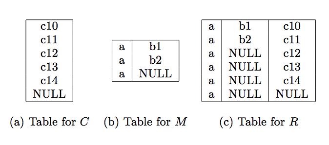
Consider the schema and the data in figure below. The values, denotes by lowercase letters, correspond to attributes with the corresponding uppercase letter.

The root in the schema has two attributes as children, M and C. In the instance, the occurrence r1 of the root has one occurrence of M and five occurrences of C. We get the union of the five occurrences of C and get the column in image (a) below. We call this relation F_C. Then we consider the instance subtree with m1 as root. Its relation, which we call F_M, is shown in (b). When we horizontally concatenate F_M and F_C, we get the semi-flattened representation for the entire instance, which is shown in (c).

Call a schema linear if the only non star free path is a single path from the root to a single leaf; we call this leaf the primary leaf.

Lemma 5.3. For any data tree in a linear schema, full flattening and semi flattening coincide.

The observation is: The only difference between the definitions of full flattening and semi-flattening is: in full flattening we have cartesian product whereas in semi flattening we have a horizontal concatenation. In the case of linear schema, the cartesian product in the definition of full flattening reduces to the horizontal concatenation in the definition of the semi-flattening.

Lemma 5.4. The schema subtree of any repetition context is a linear schema.

Lemma 5.5. If we restrict the semi-flattened data only to the columns that comprise a repetition context C (in which case, they can be thought of as being on a linear schema), then the set of rows that we get is the same as the set of rows we get if we restrict full-flattened data (of the same data tree) to repetition context C.

Theorem 5.6. Let I be an instance tree and let s-flatten(I) be the semi-flattened relation of I. Then for any query Q which uses a filter in a single repetition context the following holds:

s-flatten(Q(I)) = Q(s-flatten(I))

Aggregate Queries

The aggregate functions we consider are SUM, MAX, MIN, COUNT, AVG and COUNT-DISTINCT, under the following constraints:

1. All aggregated attributes should be dominated by all grouping attributes.
2. The SELECT clause should include only the grouping attributes and the aggregations.

Note that (1) implies that the repetition contexts of the aggregated attributes have an intersection which contains the grouping attributes. When these constraints are met in queries, we call them legitimate aggregate queries.

We give the algorithm to compute an aggregate query with grouping attribute A1 and aggregated attributed A0m where A1 dominates A0. The output will be a normal relation with two attributes, one attribute is the grouping attribute A1 and the other is a new attribute A_agg which stores the result of applying the aggregate function on bags, one bag for each value of A1. This is the description of the tree aggregating algorithm that does the computation:

1. Suppose the attribute that is LCA of A1 and A0 in the schema tree is A01. For each value u of A1, let {v1, v2, …} be all nodes in the data tree with value u, and let {v01, v02, …} be the “corresponding” values of attribute A01 (i.e., v1 has ancestor v01, v2 has ancestor v02 and so on).
2. For each value u of A1, we form a bag of values of the aggregate attribute A0. This bag stores all values for each data leaf which is a) an occurrence of A0 and b) is a descendant of a node in {v01, v02, …}.
3. Then we aggregate over the values in each bag (which corresponds to a value of A0) and store the result in the new attribute A_agg.

Of course, we need not form bags explicitly, We compute the aggregation function on the fly, except for the average function, where we need to compute both coun and sum on the fly and divide at the end and the count-distinct funciton where need ot compute a set instead of a bag.

When there is more than one grouping attribute, there is a at least one grouping attribute is dominated by all other grouping attribtues (see lemma 5.2); call one of them arbitrarily the most dominated attribute. We form one bag for each tuple of values of the grouping attributes. In this case, the computation is led by the most dominated attribute as to which subtrees we consider for all their aggregated attribute values to go in the same bag. That is, the tree-aggregating algorithm considers the LCA of the aggregated attribute and the most dominated attribute.

All legitimate aggregate queries can be conceptually computed on semi-flattened data. The way to compute them is: First NULLs are ignored. Second, for MIN and MAX we apply standard SQL semantics, However for SUM and other duplicate-sensitive aggregate functions, we need to be more careful. We observe that flattening (full or semi) may use the same data leaf in more than one rows. Thus we need to do duplicate elimination in that sense. Conceptually, this is achieved by adding a new attribute for each aggregated attribute, we call this attribute Tag. The value of Tag is either 0 (duplicate) or 1 (include this value). The value of Tag is 1 in a row of semi-flattened data if the value of the aggregated attribute in the query is the value of data leaf a and it is the first row (imagine a total order on the rows) where the value of data leaf a appears in the semi-flattened data. Otherwise it is 0. Thus, when we compute the aggregate functio, we compute it on two grouping attributes: the grouping attribute we started with and the additional one, which we constrain to have value equal to 1.

Filter and Aggregate Queries

We can also have a filter in the query but we allow comparison among the grouping attributes only. Because of Lemma 5.2 any comparison is guaranteed to be among two attributes where one of them dominates the other attribute.

The computation algorithm now, applies first the filter by using the tree pruning algorithm and in the output data tree applies the tree-aggregating algorithm to obtain the final output. Semi-flattening can be used to compute aggregate queries with filters. In following theorem, Q(I) represent the output of the query when we apply the tree pruning followed by the tree-aggregating algorithm on the data tree.

Theorem 5.7. Let I be an instance tree and s-flatten(I) be the semi-flattened relation of I. Then for any legitimate aggregate-and-filter query Q, the following holds:

Q(s-flatten(I)) = Q(I)

Efficient Data Storage and Retrieval

We have already introduced repitition level and definition level in this article. We will do a brief recap and use them to produce semi-flattened relations when reading table.

Repetition Level

The repetition level of a data leaf v is the attribute name of the LCA of v and the previous data leaf stored it its column (the previous leaf with the same attribute as v). By convention when a leaf is the first for its attribute in the record, its repetition level is root.

Below is the repetition levels of the data tree of Advertiser:

Theorem 6.1. The repetition level suffices to reconstruct the data tree if for each occurrence of an attribute, there is at least one occurrence (in the data tree) for each of its children (in the schema tree).

Producing the Semi-flattening

The algorithm by which the reader deides whether to use the current value from a column V or to move to the next value in its column is as follows:

1. As long as there is a column dominated by V whose current repetition level does not go above or at the repetition level of V, the reader for V remains in the same place and ouputs in each constructed row the current value of V.
2. Otherwise, if all its dominating attributes move to current repetition level, it goes to step 3 below. If not, it contributes NULLs (and repeats this step).
3. If V is a required attribute, the reader first produces an extra row with the current values in column V and in all the columns dominating V, whereas all other columns have NULL’s. If V is not required it doesn’t produce this row. In either case, the reader then moves to the next value in the column for V.

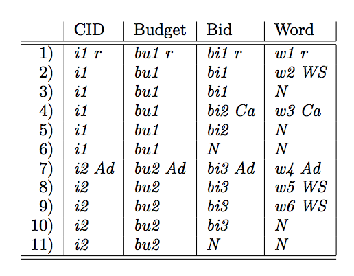
Consider the data tree for Advertiser, below is the produced semi-flattened relations with CID, Budget, Bid and Word (in dominance order). We will show how to use repetition level to produce the semi-flattening in the image. The first rwo is formed by the top elements in each column.

Producing the Second Row

The repetition level for each of the second elements in columns Bid and Word stays below (in tree context) Advertiser, which is the repetition level of the second element in columns CID and Budget. Thus these two columns stall (according to step 1 of the algorithm) and emit i1 and bu1, respectively. The second element in column Word has repetition level WordSet, which is below the repetition level of the second element in column Bid (which is Campaign). Hence for the second row, column Bid stalls too and emits bi1. Column Word is allowed by steps 1 and 2 of the algorithm to go to step 3 and make a move. Thus second row is formed.

Producing Rows 3 and 4

w3’s repetition level is Campaign, and so is teh repetition level of bi2. So, since Bid dominates Word, the column Bid can now make a move to bi2 because all its dominated columns (actually, only the one column Word) have repetition levels at or above its repetition level (step 1). Bid is required and it forms the extra row before moving to the next element (row 3 based on step 3). Row 4 includes the new value after the moves that are allowed at this stage. Columns CID and Budget still stall since the repetition levels of their next elements (i2 and bu2) are above Campaign (which is the current repetition level of some of its dominated attributes).

Producing Rows 5, 6, and 7

Next, all current (i2, bu2, bi3 and w4) repetition levels are at or above Advertiser, so columns CID, Budget and Bid move to their next element, so does column Word. Row 5 is created by the move of Bid, because it is require field (as step 3), row 6 is produced by move of CID and Budget (as step 3), their moves only produces a single row because they dominate each other. Row 7 contains new values.

Producing Rows 8, 9, 10 and 11

Rows 10 and 11 are the extra rows. Row 8 and 9 are formed by Word making one more move for each column and CID and Budget stalling.

We say that a data leaf v covers another data leaf u if the attribute V for v dominates attribute U for u, and data node u and v are descendants of the same occurrence of their LCA in the schema tree. When a data leaf convers another data leaf, the repetition level of the former is the same as or above the repetition level of the latter. For instance, b1 covers w1 and w2.

The algorithm we presented to produce semi-flattening from columnar storage only retains the covering relation. It does not care, for example, to show any interrelationship between data leaves for Fee and Word, because in the class of queries supported by semi-flattening, we do not have a query where query of Word and Fee are compared.

Finally, a note about the functionality of the extra row that the algorithm creates before a column makes a move. For example the row (i1, bu1, NULL, NULL) in the figure above. Suppose this row did not exist. Then if neither bi1 nor bi2 values of the Bid attribute satisfy the filter, the values i1 and bu1 would not appear in the result of the query. This is wrong according to the tree-pruning algorithm.

The correctness of the algorithm is a consequence of the lemma:

Lemma 6.2. If leaf v covers leaf u in the data tree, then the repetition level of u is either the same as the repetition level of v, or a decendant of the repetition level of v.

Definition Level

The definition level is a second parameter stored along with the repetition level. Its purpose is to avoid having to store NULL’s explicitly in the columns. The definition level tells how many subtrees between the current value and the previous value of the same column have zero occurrences.

Lemma 6.3. Let B be an attribute that dominates A. Let LCA(A, B) be the LCA of B and A. Suppose a data leaf v of A and a data leaf u of B occur within the same occurrence x of LCA(A, B). The repetition and the definition levels are sufficient to tell that v and u are descendants of the same occurrence of LCA(A, B).

Producing the Semi-flattening

The algorithm above is not modified so that whenever a column A is due for a move, it stalls for as many moves of star-free descendants of LCA_A as tells the definition level of A.